R Tutorials

1. Simple time series plot on ‘non-ts’ data

a. Get 200 random numbers and call the object ‘mydata’. Let’s set a seed of 14 for reproducibility.

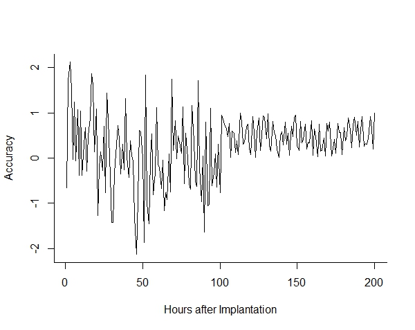
b. Get a time series plot without converting to class ‘ts’.

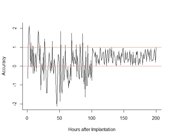
c. Add ablines to the chart to indicate the horizontal boundaries of 0 and 1.

Reveal solution

a.
set.seed(14);
mydata = c(rnorm(100), runif(100))

b.
plot.ts(mydata, bty = "l",
xlab = "Hours after Implantation",
ylab = "Accuracy")


c.
abline(h = 0, col = "salmon"); abline(h = 1, col = "salmon")

2. Working with ‘xts’

a. Get and load the package ‘xts’ and all required packages.

b. Create the objects ‘measurment’ and ‘dates’ like below.

measurement <- rep(sin(seq(0,10,length.out = 90)),4) + rnorm(90*4)

dates <- seq(as.Date("1987-01-01"), as.Date("1987-12-26"), "day")

c. Use the two objects to create an ‘xts’ time series (‘mytimeseries’) ordered by ‘dates’.

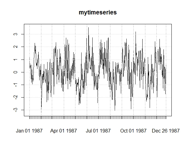
d. Plot the ‘xts’ time series.

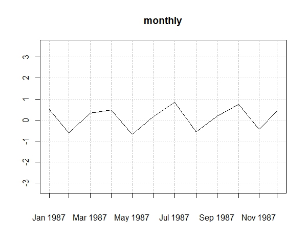
e. Use ‘apply.monthly’ from ‘xts’ to get a monthly mean on the time series.

f. Get a monthly plot.

Reveal solution

a.
install.packages("xts")
library(xts)

b.
measurement <- rep(sin(seq(0,10,length.out = 90)),4) + rnorm(90*4)
dates <- seq(as.Date("1987-01-01"), as.Date("1987-12-26"), "day")

c.
mytimeseries <- xts(measurement, order.by = dates)

d.
plot(mytimeseries)


e.
monthly <- apply.monthly(mytimeseries, mean)

f.
plot(monthly, ylim = range(mytimeseries))

3. Using ‘ts’ with different parameters

a. Create ‘mydata’ as below.

mydata = rep(sin(seq(0,10,length.out = 90)),4) + rnorm(90*4)

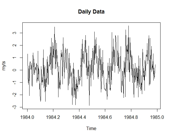
b. Create ‘myts’ which is a daily time series of ‘mydata’, starting on the second day in 1984.

c. Get a plot of ‘myts’.

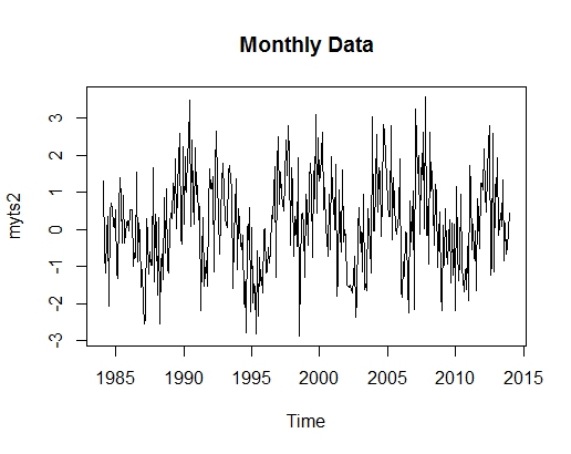
d. Create ‘myts2’ which is a monthly time series of ‘mydata’, starting in February 1984.

e. Get a plot of ‘myts2’.

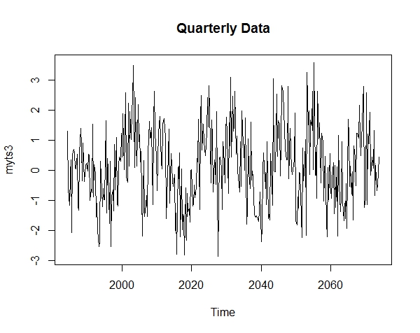
f. Create ‘myts3’ which is a quarterly time series of ‘mydata’, starting in quarter 2 of 1984.

g. Get a plot of ‘myts3’.

Reveal solution

a.
mydata = rep(sin(seq(0,10,length.out = 90)),4) + rnorm(90*4)

b.
myts = ts(mydata, start = c(1984, 2), frequency = 365)

c.
plot(myts, main = "Daily Data")


d.
myts2 = ts(mydata, start = c(1984, 2), frequency = 12)

e.
plot(myts2, main = "Monthly Data")


f.
myts3 = ts(mydata, start = c(1984, 2), frequency = 4)

g.
plot(myts3, main = "Quarterly Data")

4. Creating an object of class ‘mts’

a. Get an object ‘mydata’ as follows:

set.seed(20)

mydata1 = rnorm(500, 6)

mydata2 = rnorm(500, 77)

mydata3 = runif(500)

b. Combine the data to a data.frame ‘mydata’.

#expected result

    mydata1  mydata2     mydata3
1  7.162685 77.53992 0.520860041
2  5.414076 78.55284 0.232611279
3  7.785465 75.96940 0.795618258
4  4.667406 74.86877 0.114846902
5  5.553433 77.70767 0.639547465
6  6.569606 77.01095 0.163244763
7  3.110282 76.66075 0.992082189
8  5.130982 76.02084 0.050576476
9  5.538297 76.20912 0.421205091
10 5.444459 75.42494 0.151422651

c. Change the format to a matrix.

d. Create ‘myts’ of ‘mydata’, which starts in May 1980, this is a class ‘mts’.

5. Weekly Time Series Data – business days

a. Get 49 random numbers and call the vector ‘mydata’.

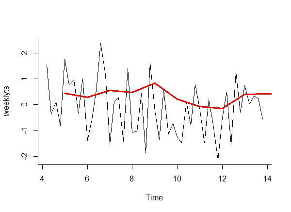
b. Convert ‘mydata’ to a weekly time series – those are five day business weeks. The time series starts on the second day of week 4. Call it ‘weeklyts’.

c. Use the function SMA from the package ‘TTR’ to get a five day simple moving average. Call the object ‘mysma’.

d. Plot the time series and add the ‘mysma’ line to the chart.

Reveal solution

a.
mydata = rnorm(49)

b.
weeklyts = ts(mydata, frequency = 5,
start=c(4, 2))

c.
install.packages("TTR")
library(TTR)

mysma = SMA(weeklyts, 5)

d.
plot(weeklyts, bty = "l")
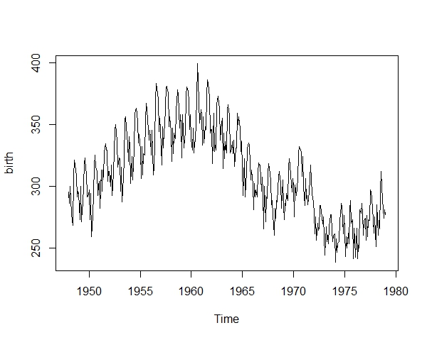
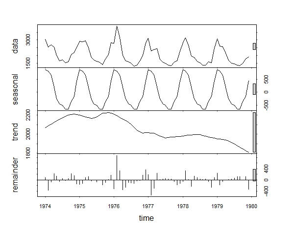
lines(mysma, col = "red", lwd = 3)

6. Decomposing the ‘birth’ dataset

a. Install and load the ‘astsa’ library and get familiar with the ‘birth’ dataset.

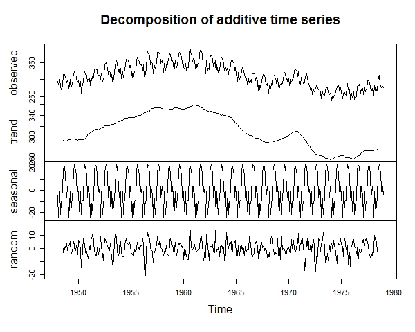
b. Get a decomposition plot of the ‘birth’ dataset.

c. Decompose the dataset and create a new object, which consists only of the components ‘seasonal’ and ‘trend’ of the original dataset. Plot the new object.

Reveal solution

a.
install.packages("astsa")
library(astsa)

head(birth); length(birth)
plot(birth)


b.
plot(decompose(birth))


c.
newbirth = decompose(birth)
trendseason = newbirth$trend + newbirth$seasonal
plot(trendseason)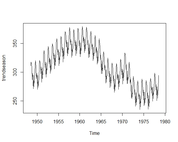

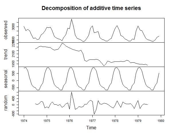
7. Different methods for decomposition

a. Use ‘decompose’ and ‘stl’ to decompose the ‘ldeaths’ dataset. Which one of the 2 functions is more customizable?

‘decompose’

‘stl’

Reveal solution

a.
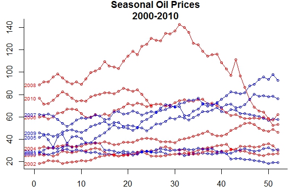
plot(decompose(ldeaths))


plot(stl(ldeaths, s.window = "periodic"))

8. Season plot

a. Install and load packages ‘forecast’ and ‘astsa’.

b. Get a season plot of the ‘oil’ dataset and tailor it in order to resemble the plot outlined here. Change the plot margins as well.

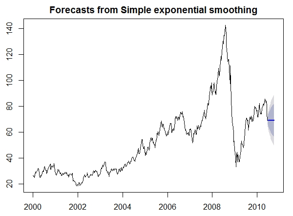
9. Forecasting with the ‘forecast’ package

a. Activate the packages ‘forecast’ and ‘astsa’.

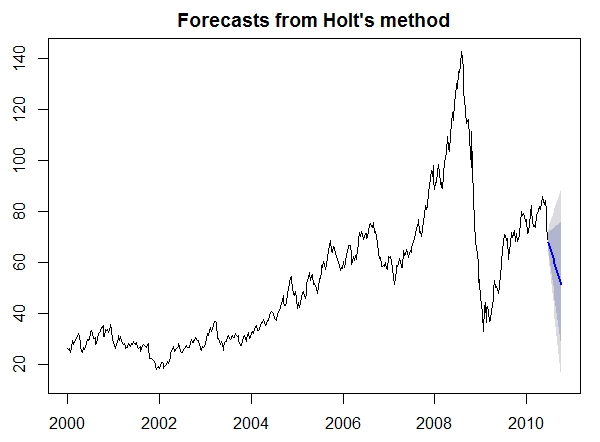
b. Use the function ‘ses’ and ‘holt’ (package ‘forecast’) to predict the next 15 weeks of the oil dataset.

c. Get a plot for each of the two prediction objects and compare the results. Which one is more trend based?.

‘ses’

‘holt’

Reveal solution

a.
library(forecast)
library(astsa)

b.
oilforecast = ses(oil, h = 15)

oilforecast2 = holt(oil, h = 15)

c.
plot(oilforecast)


plot(oilforecast2)

10. Prediction of ‘flu’ data

a. Activate libraries ‘forecast’, ‘astsa’ and ‘TTR’.

b. Use the function ‘ses’ to predict the next three months of the ‘flu’ dataset in ‘astsa’.

c. Plot the prediction and add a three months exponential moving average line to the plot.

Reveal solution

a.
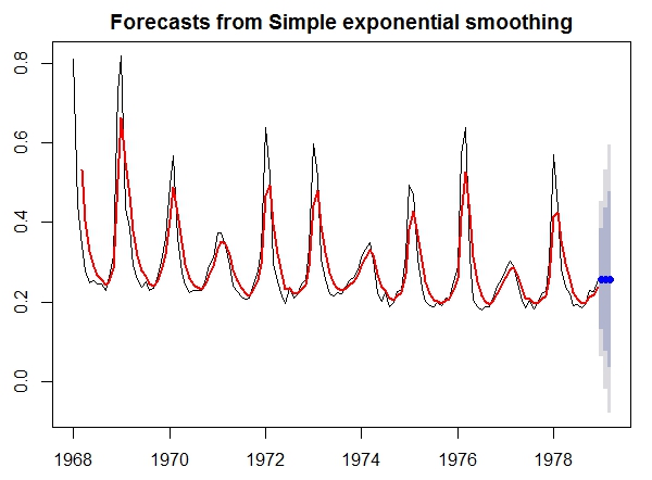
library(astsa)
library(forecast)
library(TTR)

b.
newflu = ses(flu, h = 3)

c.
plot(newflu)
lines(EMA(flu, n = 3), col = "red", lwd = 2)