R Exercises – 31-40 – Data Frame Manipulations
1. Working with the ‘mtcars’ dataset
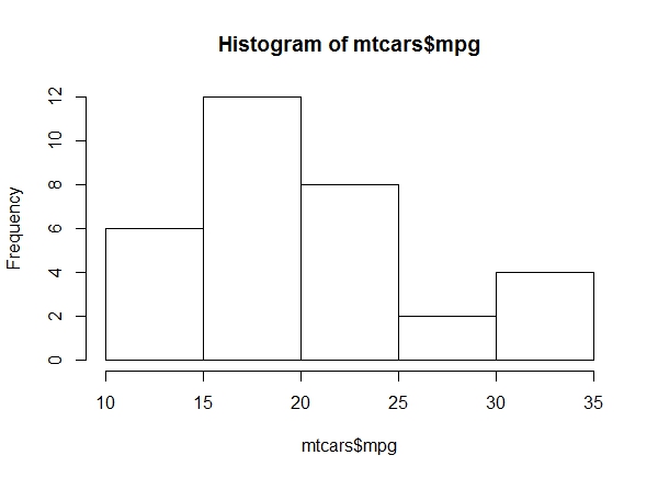
a. Get a histogram of the ‘mpg’ values of ‘mtcars’. Which bin contains the most observations?
b. Are there more automatic (0) or manual (1) transmission-type cars in the dataset? Hint: ‘mtcars’ has 32 observations.
c. Get a scatter plot of ‘hp’ vs ‘weight’.
hist(mtcars$mpg)Bin 15-20
b.
sum(mtcars$am == 1)

sum(mtcars$am == 0)
There are more automatic (0) cars.
c.
plot(mtcars$wt, mtcars$hp, col = "red", pch = 3,

bty = "l", xlab = "Car Weight in 1K lbs", ylab = "Horsepower" )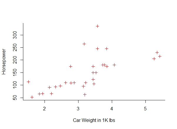
2. Working with the ‘iris’ dataset
a. Get all rows of Species ‘versicolor’ in a new data frame. Call this data frame: ‘iris.vers’
#expected result

   Sepal.Length Sepal.Width Petal.Length Petal.Width    Species
51          7.0         3.2          4.7         1.4 versicolor
52          6.4         3.2          4.5         1.5 versicolor
53          6.9         3.1          4.9         1.5 versicolor
54          5.5         2.3          4.0         1.3 versicolor
55          6.5         2.8          4.6         1.5 versicolor
56          5.7         2.8          4.5         1.3 versicolor
57          6.3         3.3          4.7         1.6 versicolor
58          4.9         2.4          3.3         1.0 versicolor
59          6.6         2.9          4.6         1.3 versicolor
60          5.2         2.7          3.9         1.4 versicolor
b. Get a vector called ‘sepal.dif’ with the difference between ‘Sepal.Length’ and ‘Sepal.Width’ of ‘versicolor’ plants.
#expected result

[1]  3.8 3.2 3.8 3.2 3.7 2.9 3.0 2.5 3.7 2.5 3.0 2.9 3.8 3.2 2.7 3.6 2.6 3.1 4.0
[20] 3.1 2.7 3.3 3.8 3.3 3.5 3.6 4.0 3.7 3.1 3.1 3.1 3.1 3.1 3.3 2.4 2.6 3.6 4.0
[39] 2.6 3.0 2.9 3.1 3.2 2.7 2.9 2.7 2.8 3.3 2.6 2.9
c. Update (add) ‘iris.vers’ with the new column ‘sepal.dif’.
#expected result

   Sepal.Length Sepal.Width Petal.Length Petal.Width    Species sepal.dif
51          7.0         3.2          4.7         1.4 versicolor       3.8
52          6.4         3.2          4.5         1.5 versicolor       3.2
53          6.9         3.1          4.9         1.5 versicolor       3.8
54          5.5         2.3          4.0         1.3 versicolor       3.2
55          6.5         2.8          4.6         1.5 versicolor       3.7
56          5.7         2.8          4.5         1.3 versicolor       2.9
iris.vers = subset(iris, Species == "versicolor"); iris.versb.
sepal.dif = iris.vers$Sepal.Length - iris.vers$Sepal.Width; sepal.difc.
iris.vers = data.frame(iris.vers, sepal.dif); head(iris.vers) 3. Classes of Variables (‘mtcars’)
a. Check the class of each variable in ‘mtcars’.
#expected result

      mpg       cyl      disp        hp      drat        wt      qsec        vs
"numeric" "numeric" "numeric" "numeric" "numeric" "numeric" "numeric" "numeric"

       am      gear      carb
"numeric" "numeric" "numeric"
b. Change ‘am’, ‘cyl’ and ‘vs’ to integer and store the new dataset as ‘newmtc’.
#expected result

       mpg as.integer.cyl.     disp         hp      drat
 "numeric"       "integer" "numeric" "numeric" "numeric"

        wt      qsec as.integer.vs. as.integer.am.      gear
 "numeric" "numeric"      "integer"      "integer" "numeric"

      carb
 "numeric"
c. Round the ‘newmtc’ data frame to one digit.
#expected result

    mpg as.integer.cyl.  disp  hp drat  wt qsec as.integer.vs. as.integer.am. gear carb
1  21.0               6 160.0 110  3.9 2.6 16.5              0              1    4    4
2  21.0               6 160.0 110  3.9 2.9 17.0              0              1    4    4
3  22.8               4 108.0  93  3.8 2.3 18.6              1              1    4    1
4  21.4               6 258.0 110  3.1 3.2 19.4              1              0    3    1
5  18.7               8 360.0 175  3.1 3.4 17.0              0              0    3    2
6  18.1               6 225.0 105  2.8 3.5 20.2              1              0    3    1
7  14.3               8 360.0 245  3.2 3.6 15.8              0              0    3    4
8  24.4               4 146.7  62  3.7 3.2 20.0              1              0    4    2
9  22.8               4 140.8  95  3.9 3.1 22.9              1              0    4    2
10 19.2               6 167.6 123  3.9 3.4 18.3              1              0    4    4
head(mtcars)

sapply(mtcars, class)
b.
attach(mtcars)

newmtc = data.frame(mpg, as.integer(cyl), disp, hp, drat, wt, qsec,

as.integer(vs), as.integer(am), gear, carb)

sapply(newmtc, class)
c.
round(newmtc, 1) 4. Advanced filtering of ‘iris’
a. Use ‘dplyr’ to filter for all data of Species ‘virginica’ with a ‘Sepal.Width’ of greater than 3.5.
#expected result

  Sepal.Length Sepal.Width Petal.Length Petal.Width   Species
1          7.2         3.6          6.1         2.5 virginica
2          7.7         3.8          6.7         2.2 virginica
3          7.9         3.8          6.4         2.0 virginica
b. How would you use R Base to get a data frame of all data of Species ‘virginica’ with a ‘Sepal.Width’ of greater than 3.5, but without the last column Species in the data frame?
#expected result

    Sepal.Length Sepal.Width Petal.Length Petal.Width
110          7.2         3.6          6.1         2.5
118          7.7         3.8          6.7         2.2
132          7.9         3.8          6.4         2.0
c. Get the row IDs of the rows matching the two filtering criteria provided above.
#expected result

[1] "110" "118" "132"
library(dplyr)

filter(iris, Sepal.Width > 3.5, Species =="virginica")
b.
iris[iris$Species == "virginica" & iris$Sepal.Width > 3.5, 1:4]c.
row.names(iris[iris$Species == "virginica" & iris$Sepal.Width > 3.5, 1:4]) 5. Manipulating data frames at column level (dataset = ‘iris’)
a. Repeat each value of ‘Sepal.Length’ two times and repeat the whole sequence two times as well.
#expected result

[1]   5.1 5.1 4.9 4.9 4.7 4.7 4.6 4.6 5.0 5.0 5.4 5.4 4.6 4.6 5.0 5.0 4.4 4.4 4.9 4.9 5.4 5.4 4.8
[24]  4.8 4.8 4.8 4.3 4.3 5.8 5.8 5.7 5.7 5.4 5.4 5.1 5.1 5.7 5.7 5.1 5.1 5.4 5.4 5.1 5.1 4.6 4.6
[47]  5.1 5.1 4.8 4.8 5.0 5.0 5.0 5.0 5.2 5.2 5.2 5.2 4.7 4.7 4.8 4.8 5.4 5.4 5.2 5.2 5.5 5.5 4.9
[70]  4.9 5.0 5.0 5.5 5.5 4.9 4.9 4.4 4.4 5.1 5.1 5.0 5.0 4.5 4.5 4.4 4.4 5.0 5.0 5.1 5.1 4.8 4.8
[93]  5.1 5.1 4.6 4.6 5.3 5.3 5.0 5.0 7.0 7.0 6.4 6.4 6.9 6.9 5.5 5.5 6.5 6.5 5.7 5.7 6.3 6.3 4.9
[116] 4.9 6.6 6.6 5.2 5.2 5.0 5.0 5.9 5.9 6.0 6.0 6.1 6.1 5.6 5.6 6.7 6.7 5.6 5.6 5.8 5.8 6.2 6.2
[139] 5.6 5.6 5.9 5.9 6.1 6.1 6.3 6.3 6.1 6.1 6.4 6.4 6.6 6.6 6.8 6.8 6.7 6.7 6.0 6.0 5.7 5.7 5.5
[162] 5.5 5.5 5.5 5.8 5.8 6.0 6.0 5.4 5.4 6.0 6.0 6.7 6.7 6.3 6.3 5.6 5.6 5.5 5.5 5.5 5.5 6.1 6.1
[185] 5.8 5.8 5.0 5.0 5.6 5.6 5.7 5.7 5.7 5.7 6.2 6.2 5.1 5.1 5.7 5.7 6.3 6.3 5.8 5.8 7.1 7.1 6.3
[208] 6.3 6.5 6.5 7.6 7.6 4.9 4.9 7.3 7.3 6.7 6.7 7.2 7.2 6.5 6.5 6.4 6.4 6.8 6.8 5.7 5.7 5.8 5.8
[231] 6.4 6.4 6.5 6.5 7.7 7.7 7.7 7.7 6.0 6.0 6.9 6.9 5.6 5.6 7.7 7.7 6.3 6.3 6.7 6.7 7.2 7.2 6.2
[254] 6.2 6.1 6.1 6.4 6.4 7.2 7.2 7.4 7.4 7.9 7.9 6.4 6.4 6.3 6.3 6.1 6.1 7.7 7.7 6.3 6.3 6.4 6.4
[277] 6.0 6.0 6.9 6.9 6.7 6.7 6.9 6.9 5.8 5.8 6.8 6.8 6.7 6.7 6.7 6.7 6.3 6.3 6.5 6.5 6.2 6.2 5.9
[300] 5.9 5.1 5.1 4.9 4.9 4.7 4.7 4.6 4.6 5.0 5.0 5.4 5.4 4.6 4.6 5.0 5.0 4.4 4.4 4.9 4.9 5.4 5.4
[323] 4.8 4.8 4.8 4.8 4.3 4.3 5.8 5.8 5.7 5.7 5.4 5.4 5.1 5.1 5.7 5.7 5.1 5.1 5.4 5.4 5.1 5.1 4.6
[346] 4.6 5.1 5.1 4.8 4.8 5.0 5.0 5.0 5.0 5.2 5.2 5.2 5.2 4.7 4.7 4.8 4.8 5.4 5.4 5.2 5.2 5.5 5.5
[369] 4.9 4.9 5.0 5.0 5.5 5.5 4.9 4.9 4.4 4.4 5.1 5.1 5.0 5.0 4.5 4.5 4.4 4.4 5.0 5.0 5.1 5.1 4.8
[392] 4.8 5.1 5.1 4.6 4.6 5.3 5.3 5.0 5.0 7.0 7.0 6.4 6.4 6.9 6.9 5.5 5.5 6.5 6.5 5.7 5.7 6.3 6.3
[415] 4.9 4.9 6.6 6.6 5.2 5.2 5.0 5.0 5.9 5.9 6.0 6.0 6.1 6.1 5.6 5.6 6.7 6.7 5.6 5.6 5.8 5.8 6.2
[438] 6.2 5.6 5.6 5.9 5.9 6.1 6.1 6.3 6.3 6.1 6.1 6.4 6.4 6.6 6.6 6.8 6.8 6.7 6.7 6.0 6.0 5.7 5.7
[461] 5.5 5.5 5.5 5.5 5.8 5.8 6.0 6.0 5.4 5.4 6.0 6.0 6.7 6.7 6.3 6.3 5.6 5.6 5.5 5.5 5.5 5.5 6.1
[484] 6.1 5.8 5.8 5.0 5.0 5.6 5.6 5.7 5.7 5.7 5.7 6.2 6.2 5.1 5.1 5.7 5.7 6.3 6.3 5.8 5.8 7.1 7.1
[507] 6.3 6.3 6.5 6.5 7.6 7.6 4.9 4.9 7.3 7.3 6.7 6.7 7.2 7.2 6.5 6.5 6.4 6.4 6.8 6.8 5.7 5.7 5.8
[530] 5.8 6.4 6.4 6.5 6.5 7.7 7.7 7.7 7.7 6.0 6.0 6.9 6.9 5.6 5.6 7.7 7.7 6.3 6.3 6.7 6.7 7.2 7.2
[553] 6.2 6.2 6.1 6.1 6.4 6.4 7.2 7.2 7.4 7.4 7.9 7.9 6.4 6.4 6.3 6.3 6.1 6.1 7.7 7.7 6.3 6.3 6.4
[576] 6.4 6.0 6.0 6.9 6.9 6.7 6.7 6.9 6.9 5.8 5.8 6.8 6.8 6.7 6.7 6.7 6.7 6.3 6.3 6.5 6.5 6.2 6.2
[599] 5.9 5.9
b. Get a new object which contains only the odd values of ‘Sepal.Length’.
#expected result

[1]  5.1 4.7 5.0 4.6 4.4 5.4 4.8 5.8 5.4 5.7 5.4 4.6 4.8 5.0 5.2 4.8 5.2 4.9 5.5 4.4 5.0 4.4 5.1
[24] 5.1 5.3 7.0 6.9 6.5 6.3 6.6 5.0 6.0 5.6 5.6 6.2 5.9 6.3 6.4 6.8 6.0 5.5 5.8 5.4 6.7 5.6 5.5
[47] 5.8 5.6 5.7 5.1 6.3 7.1 6.5 4.9 6.7 6.5 6.8 5.8 6.5 7.7 6.9 7.7 6.7 6.2 6.4 7.4 6.4 6.1 6.3
[70] 6.0 6.7 5.8 6.7 6.3 6.2
c. Get a new object which repeats each value from the new vector of exercise b.
#expected result

[1]   5.1 5.1 4.7 4.7 5.0 5.0 4.6 4.6 4.4 4.4 5.4 5.4 4.8 4.8 5.8 5.8 5.4 5.4 5.7 5.7 5.4 5.4 4.6
[24]  4.6 4.8 4.8 5.0 5.0 5.2 5.2 4.8 4.8 5.2 5.2 4.9 4.9 5.5 5.5 4.4 4.4 5.0 5.0 4.4 4.4 5.1 5.1
[47]  5.1 5.1 5.3 5.3 7.0 7.0 6.9 6.9 6.5 6.5 6.3 6.3 6.6 6.6 5.0 5.0 6.0 6.0 5.6 5.6 5.6 5.6 6.2
[70]  6.2 5.9 5.9 6.3 6.3 6.4 6.4 6.8 6.8 6.0 6.0 5.5 5.5 5.8 5.8 5.4 5.4 6.7 6.7 5.6 5.6 5.5 5.5
[93]  5.8 5.8 5.6 5.6 5.7 5.7 5.1 5.1 6.3 6.3 7.1 7.1 6.5 6.5 4.9 4.9 6.7 6.7 6.5 6.5 6.8 6.8 5.8
[116] 5.8 6.5 6.5 7.7 7.7 6.9 6.9 7.7 7.7 6.7 6.7 6.2 6.2 6.4 6.4 7.4 7.4 6.4 6.4 6.1 6.1 6.3 6.3
[139] 6.0 6.0 6.7 6.7 5.8 5.8 6.7 6.7 6.3 6.3 6.2 6.2
d. Replace the ‘Sepal.Length’ column of ‘iris’ with the new ‘Sepal.Length’ from exercise c. Check if the replacement worked.
#expected result

   Sepal.Length Sepal.Width Petal.Length Petal.Width Species
1           5.1         3.5          1.4         0.2  setosa
2           5.1         3.0          1.4         0.2  setosa
3           4.7         3.2          1.3         0.2  setosa
4           4.7         3.1          1.5         0.2  setosa
5           5.0         3.6          1.4         0.2  setosa
6           5.0         3.9          1.7         0.4  setosa
rep(iris$Sepal.Length, each = 2, times = 2)b.
sep.lengthodd = iris[c(T,F),1]c.
newsep.length = rep(sep.lengthodd, each = 2)d.
iris$Sepal.Length = newsep.length; head(iris) 6. Big Data Example with ‘diamonds’ (package: ‘ggplot2’)
a. Get familiar with the dataset ‘diamonds’ from ‘ggplot2’.
b. Attach the dataset.
c. Get a subset from the diamonds dataset with all the rows that have a clarity of ‘SI2’ and a depth of at least 70. Call the subset ‘diam.sd’ and display it in the same line of code.
#expected result

# A tibble: 6 x 10
   carat   cut color clarity depth table price     x     y     z
   <dbl> <ord> <ord>   <ord> <dbl> <dbl> <int> <dbl> <dbl> <dbl>
1   1.50  Fair     I     SI2  70.1    58  4328  6.96  6.85  4.84
2   2.00  Fair     F     SI2  70.2    57 15351  7.63  7.59  5.34
3   0.70  Fair     D     SI2  71.6    55  1696  5.47  5.28  3.85
4   0.70  Fair     E     SI2  70.6    56  1828  5.45  5.35  3.81
5   1.00  Fair     G     SI2  70.2    58  2326  6.00  5.73  4.13
6   0.96  Fair     G     SI2  72.2    56  2438  6.01  5.81  4.28
d. Which index positions have a clarity of ‘SI2’ and a depth of at least 70? (hint: ‘row.names’)
#expected result

[1] "1" "2" "3" "4" "5" "6"
e. Store the index positions as an integer object.
#expected result

[1] 1 2 3 4 5 6
library(ggplot2)

? diamonds

summary(diamonds)
b.
attach(diamonds)c.
diam.sd = subset(diamonds, clarity == "SI2" & depth >= 70); diam.sdd.
row.names(diam.sd)e.
index.pos = as.integer(row.names(diam.sd)); index.pos 7. Getting counts of filtered datasets (‘ggplot2’ : ‘diamonds’)
a. How many observations of diamonds have a cut of ‘ideal’ and have less than 0.21 carat?
b. How many observations of diamonds have a combined ‘x’ + ‘y’ + ‘z’ dimension greater than 40?
c. How many observations of diamonds have either a price above 10.000 USD or a depth of at least 70?
sum(cut == "Ideal" & carat < 0.21)'diamonds' is attached to environment
b.
sum ((x + y + z) > 40)c.
sum(price > 10000 | depth >= 70) 8. Filtering based on row and column ID (‘ggplot2’: ‘diamonds’)
a. Get a data frame with observations ’67’ and ‘982’ of variables color and y.
#expected result

# A tibble: 2 x 2
  color     y
  <ord> <dbl>
1     I  4.42
2     F  5.76
b. Get a data frame with the full info on observations ‘453’, ‘792’ and ‘10489’.
#expected result

# A tibble: 3 x 10
   carat       cut color clarity depth table price     x     y     z
   <dbl>     <ord> <ord>   <ord> <dbl> <dbl> <int> <dbl> <dbl> <dbl>
1   0.71     Ideal     I    VVS2  60.2    56  2817  5.84  5.89  3.53
2   0.70 Very Good     D     SI1  62.5    55  2862  5.67  5.72  3.56
3   1.01     Ideal     F     SI2  60.0    57  4796  6.55  6.51  3.92
c. Get the first 10 rows of the dataset ‘diamonds’ with the variables ‘x’, ‘y’, ‘z’.
#expected result

# A tibble: 10 x 3
      x     y     z
  <dbl> <dbl> <dbl>
1  3.95  3.98  2.43
2  3.89  3.84  2.31
3  4.05  4.07  2.31
4  4.20  4.23  2.63
5  4.34  4.35  2.75
6  3.94  3.96  2.48
7  3.95  3.98  2.47
8  4.07  4.11  2.53
9  3.87  3.78  2.49
10 4.00  4.05  2.39
d. Get the first six values of ‘diamonds’ of the variable ‘y’ as a simple vector.
#expected result

# A tibble: 6 x 1
      y
  <dbl>
1  3.98
2  3.84
3  4.07
4  4.23
5  4.35
6  3.96
diamonds[c(67,982), c(3,9)]b.
diamonds[c(453, 792, 10489), ]c.
head(diamonds[ , c(8,9,10)],10)d.
head(diamonds[,"y"])different output format: 'vector'
9. Ordering data (‘ggplot2’: ‘diamonds’)
a. Create the object ‘newdiam’ which is a subset of the first 1000 rows of ‘diamonds’.
#expected result

# A tibble: 1,000 x 10
  carat       cut color clarity depth table price     x     y     z
  <dbl>     <ord> <ord>   <ord> <dbl> <dbl> <int> <dbl> <dbl> <dbl>
1  0.23     Ideal     E     SI2  61.5    55   326  3.95  3.98  2.43
2  0.21   Premium     E     SI1  59.8    61   326  3.89  3.84  2.31
3  0.23      Good     E     VS1  56.9    65   327  4.05  4.07  2.31
4  0.29   Premium     I     VS2  62.4    58   334  4.20  4.23  2.63
5  0.31      Good     J     SI2  63.3    58   335  4.34  4.35  2.75
6  0.24 Very Good     J    VVS2  62.8    57   336  3.94  3.96  2.48
7  0.24 Very Good     I    VVS1  62.3    57   336  3.95  3.98  2.47
b. Order ‘newdiam’ according to price, starting with the lowest. Hint: ‘dplyr’, ‘arrange’ is a useful function for that.
#expected result

# A tibble: 6 x 10
  carat       cut color clarity depth table price     x     y     z
  <dbl>     <ord> <ord>   <ord> <dbl> <dbl> <int> <dbl> <dbl> <dbl>
1  0.23     Ideal     E     SI2  61.5    55   326  3.95  3.98  2.43
2  0.21   Premium     E     SI1  59.8    61   326  3.89  3.84  2.31
3  0.23      Good     E     VS1  56.9    65   327  4.05  4.07  2.31
4  0.29   Premium     I     VS2  62.4    58   334  4.20  4.23  2.63
5  0.31      Good     J     SI2  63.3    58   335  4.34  4.35  2.75
6  0.24 Very Good     J    VVS2  62.8    57   336  3.94  3.96  2.48
c. Order ‘newdiam’ according to price, starting with the highest.
#expected result

# A tibble: 6 x 10
  carat       cut color clarity depth table price     x     y     z
  <dbl>     <ord> <ord>   <ord> <dbl> <dbl> <int> <dbl> <dbl> <dbl>
1  1.12   Premium     J     SI2  60.6    59  2898  6.68  6.61  4.03
2  0.60 Very Good     D    VVS2  60.6    57  2897  5.48  5.51  3.33
3  0.76   Premium     E     SI1  61.1    58  2897  5.91  5.85  3.59
4  0.54     Ideal     D    VVS2  61.4    52  2897  5.30  5.34  3.26
5  0.72     Ideal     E     SI1  62.5    55  2897  5.69  5.74  3.57
6  0.72      Good     F     VS1  59.4    61  2897  5.82  5.89  3.48
d. Order ‘newdiam’ like in exercise c, but ties should be arranged with increasing depth.
#expected result

# A tibble: 6 x 10
  carat       cut color clarity depth table price     x     y     z
  <dbl>     <ord> <ord>   <ord> <dbl> <dbl> <int> <dbl> <dbl> <dbl>
1  1.12   Premium     J     SI2  60.6    59  2898  6.68  6.61  4.03
2  0.72      Good     F     VS1  59.4    61  2897  5.82  5.89  3.48
3  0.60 Very Good     D    VVS2  60.6    57  2897  5.48  5.51  3.33
4  0.76   Premium     E     SI1  61.1    58  2897  5.91  5.85  3.59
5  0.54     Ideal     D    VVS2  61.4    52  2897  5.30  5.34  3.26
6  0.74   Premium     D     VS2  61.8    58  2897  5.81  5.77  3.58
newdiam = diamonds[1:1000,]b.
library(dplyr)

head(arrange(newdiam, price))
c.
head(arrange(newdiam, desc(price)))d.
head(arrange(newdiam, desc(price), depth)) 10. Sampling big data frames (‘ggplot2’: ‘diamonds’)
a. Use ‘dplyr’, ‘sample_n’ to get the object ‘diam750’ which contains 750 randomly sampled observations of ‘diamonds’. I use seed nr. 56 for reproduction.
#expected result

# A tibble: 750 x 10
  carat       cut color clarity depth table price     x     y     z
  <dbl>     <ord> <ord>   <ord> <dbl> <dbl> <int> <dbl> <dbl> <dbl>
1  1.50     Ideal     I     VS1  61.3    57  9900  7.32  7.35  4.50
2  0.33     Ideal     E    VVS1  60.2    57  1052  4.50  4.47  2.70
3  1.02   Premium     F     VS2  62.4    59  6652  6.40  6.45  4.01
4  0.41   Premium     F     VS1  62.6    58  1076  4.75  4.74  2.97
5  1.08   Premium     F     VS2  62.1    59  7637  6.59  6.54  4.08
6  1.01   Premium     I     SI2  62.6    55  3818  6.43  6.38  4.01
7  1.05 Very Good     G     SI1  59.7    58  5019  6.60  6.66  3.96
8  1.00     Ideal     F     SI2  61.2    57  4452  6.48  6.39  3.94
9  0.55   Premium     H     SI2  59.8    59  1011  5.33  5.30  3.18
10 2.51      Fair     H     SI2  64.7    57 18308  8.44  8.50  5.48
# ... with 740 more rows
b. Get a summary of the new data frame.
#expected result

     carat               cut    color     clarity      depth           table
 Min.   :0.2300      Fair : 25  D: 73    SI1  :171  Min.   :56.70  Min.   :53.00
 1st Qu.:0.4000      Good : 70  E:144    VS2  :154  1st Qu.:61.00  1st Qu.:56.00
 Median :0.7050  Very Good:182  F:128    SI2  :141  Median :61.80  Median :57.00
 Mean   :0.8192   Premium :187  G:169    VS1  :120  Mean   :61.77  Mean   :57.51
 3rd Qu.:1.0500     Ideal :286  H:127    VVS2 : 72  3rd Qu.:62.60  3rd Qu.:59.00
 Max.   :4.1300                 I: 65    VVS1 : 56  Max.   :69.70  Max.   :67.00
                                J: 44  (Other): 36

       price             x               y              z
 Min.   :  361.0  Min.   : 3.910  Min.   :3.960  Min.   :0.000
 1st Qu.:  982.2  1st Qu.: 4.700  1st Qu.:4.710  1st Qu.:2.913
 Median : 2385.5  Median : 5.700  Median :5.705  Median :3.535
 Mean   : 4066.9  Mean   : 5.765  Mean   :5.766  Mean   :3.556
 3rd Qu.: 5400.8  3rd Qu.: 6.548  3rd Qu.:6.555  3rd Qu.:4.050
 Max.   :18804.0  Max.   :10.000  Max.   :9.850  Max.   :6.430
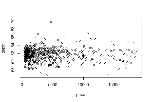
c. Plot a scatter plot of price vs depth. Use R Base plot, and the function ‘with’ (less code).
library(dplyr)

set.seed(56)

diam750 = sample_n(diamonds, 750)
b.
summary(diam750)c.
with(diam750, plot(price, depth))