
R Exercises – 21-30 – The Apply Family of Functions
1. Function ‘apply’ on a simple matrix:
a. Get the following matrix of 5 rows and call it ‘mymatrix’
mymatrix = matrix(data = c(6,34,923,5,0, 112:116, 5,9,34,76,2, 545:549), nrow = 5)
mymatrix

    [,1] [,2] [,3] [,4]
[1,]   6  112    5  545
[2,]  34  113    9  546
[3,] 923  114   34  547
[4,]   5  115   76  548
[5,]   0  116    2  549
b. Get the mean of each row
#expected result

[1] 167.00 175.50 404.50 186.00 166.75
c. Get the mean of each column
#expected result

[1] 193.6 114.0 25.2 547.0
d. Sort the columns in ascending order
#expected result

    [,1] [,2] [,3] [,4]
[1,]   0  112    2  545
[2,]   5  113    5  546
[3,]   6  114    9  547
[4,]  34  115   34  548
[5,] 923  116   76  549
mymatrix = matrix(data = c(6,34,923,5,0, 112:116, 5,9,34,76,2, 545:549), nrow = 5)b.
apply(mymatrix, MARGIN = 1, FUN = mean)c.
apply(mymatrix, MARGIN = 2, FUN = mean)d.
apply(mymatrix, MARGIN = 2, FUN = sort)2. Using ‘lapply’ on a data.frame ‘mtcars’
a. Use three ‘apply’ family functions to get the minimum values of each column of the ‘mtcars’ dataset (hint: ‘lapply’, ‘sapply’, ‘mapply’).
Store each output in a separate object (‘l’, ‘s’, ‘m’) and get the outputs.
#expected result

>l
$mpg
[1] 10.4

$cyl
[1] 4

$disp
[1] 71.1

$hp
[1] 52

$drat
[1] 2.76

$wt
[1] 1.513

$qsec
[1] 14.5

$vs
[1] 0

$am
[1] 0

$gear
[1] 3

$carb
[1] 1

>s
   mpg   cyl   disp     hp  drat    wt   qsec    vs    am  gear  carb
10.400 4.000 71.100 52.000 2.760 1.513 14.500 0.000 0.000 3.000 1.000

>m
   mpg   cyl   disp     hp  drat    wt   qsec    vs    am  gear  carb
10.400 4.000 71.100 52.000 2.760 1.513 14.500 0.000 0.000 3.000 1.000
b. Put the three outputs ‘l’, ‘s’, ‘m’ in the list ‘listobjects’
c. Use a suitable ‘apply’ function to get the class of each of the three list elements in ‘listobjects’
d. Name the output classes for each of the three functions used in the exercise
lapply(mtcars, FUN = min) -> l

sapply(mtcars, FUN = min) -> s

mapply(mtcars, FUN = min) -> m

l; s; m
b.
listobjects = list(l, s, m)c.
sapply(FUN = class, X = listobjects)d.
'lapply' gives a list,
'sapply' and 'mapply' give vectors per default
3. ‘mapply’
a. Use ‘mapply’ to get a list of 10 elements. The list is an alteration of ‘A’ and ‘F’. The lengths of those 10 alternating elements decreases step by step from 10 to 1.
#expected result

$A
 [1] "A" "A" "A" "A" "A" "A" "A" "A" "A" "A"

$F
[1] "F" "F" "F" "F" "F" "F" "F" "F" "F"

$<NA>
[1] "A" "A" "A" "A" "A" "A" "A" "A"

$<NA>
[1] "F" "F" "F" "F" "F" "F" "F"

$<NA>
[1] "A" "A" "A" "A" "A" "A"

$<NA>
[1] "F" "F" "F" "F" "F"

$<NA>
[1] "A" "A" "A" "A"

$<NA>
[1] "F" "F" "F"

$<NA>
[1] "A" "A"

$<NA>
[1] "F"
b. Tweak the function that you get proper element numbers (1 : 10) for the 10 list elements. Hint: argument USE.NAMES
#expected result

[[1]]
 [1] "A" "A" "A" "A" "A" "A" "A" "A" "A" "A"

[[2]]
[1] "F" "F" "F" "F" "F" "F" "F" "F" "F"

[[3]]
[1] "A" "A" "A" "A" "A" "A" "A" "A"

[[4]]
[1] "F" "F" "F" "F" "F" "F" "F"

[[5]]
[1] "A" "A" "A" "A" "A" "A"

[[6]]
[1] "F" "F" "F" "F" "F"

[[7]]
[1] "A" "A" "A" "A"

[[8]]
[1] "F" "F" "F"

[[9]]
[1] "A" "A"

[[10]]
[1] "F"
mapply(rep, c("A", "F"), 10:1)b.
mapply(rep, c("A", "F"), 10:1, USE.NAMES = F)

#proper element numbers
4. Titanic Casualties – Use the standard ‘Titanic’ dataset which is part of R Base
a. Use an appropriate apply function to get the sum of males vs females aboard.
#expected result

Male Female
 1731 470
b. Get a table with the sum of survivors vs sex.
#expected result

       Survived
 Sex     No Yes
 Male  1364 367
 Female 126 344
c. Get a table with the sum of passengers by sex vs age.
#expected result

           Sex
   Age  Male Female
 Child    64     45
 Adult  1667    425
apply(Titanic, 2, sum)b.
apply(Titanic, c(2,4), sum)c.
apply(Titanic, c(3,2), sum) 5. Extracting elements from a list of matrices with ‘lapply’
a. Create ‘listobj’ which is a list of four matrices – see data:
first = matrix(38:66, 3)
second = matrix(56:91, 3)
third = matrix(82:145, 3)
fourth = matrix(46:93, 5)
listobj = list(first, second, third, fourth)
b. Extract the second column from the list of matrices (from each single matrix).
#expected result

[[1]]
[1] 41 42 43

[[2]]
[1] 59 60 61

[[3]]
[1] 85 86 87

[[4]]
[1] 51 52 53 54 55
c. Extract the third row from the list of matrices.
#expected result

[[1]]
 [1] 40 43 46 49 52 55 58 61 64 38

[[2]]
 [1] 58 61 64 67 70 73 76 79 82 85 88 91

[[3]]
 [1] 84 87 90 93 96 99 102 105 108 111 114 117 120 123 126 129 132 135 138 141 144 83

[[4]]
 [1] 48 53 58 63 68 73 78 83 88 93
first = matrix(38:66, 3)

second = matrix(56:91, 3)

third = matrix(82:145, 3)

fourth = matrix(46:93, 5)

listobj = list(first, second, third, fourth)
b.
lapply(listobj,"[", , 2)c.
lapply(listobj,"[", 3 , ) 6. Plotting with the ‘apply’ family. Use the dataset ‘iris’ from R Base.
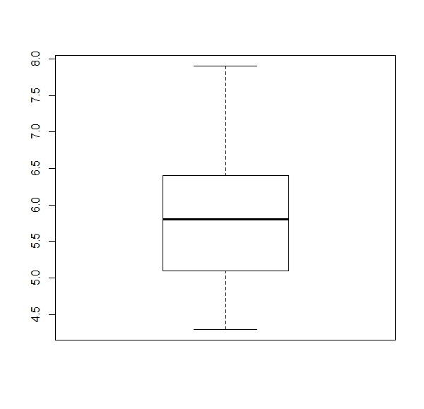
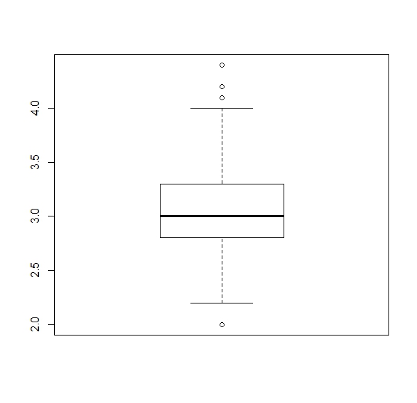
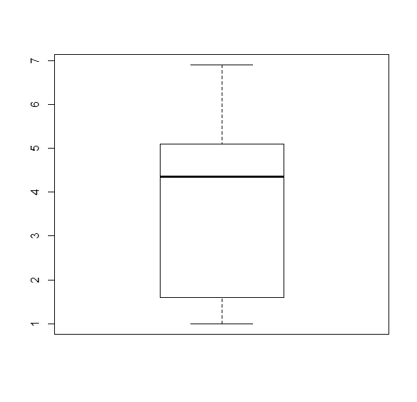
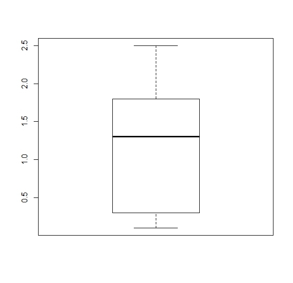
a. Get a boxplot for each numerical column of the ‘iris’ dataset (four boxplots).
Expected results:
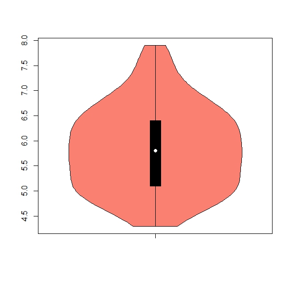
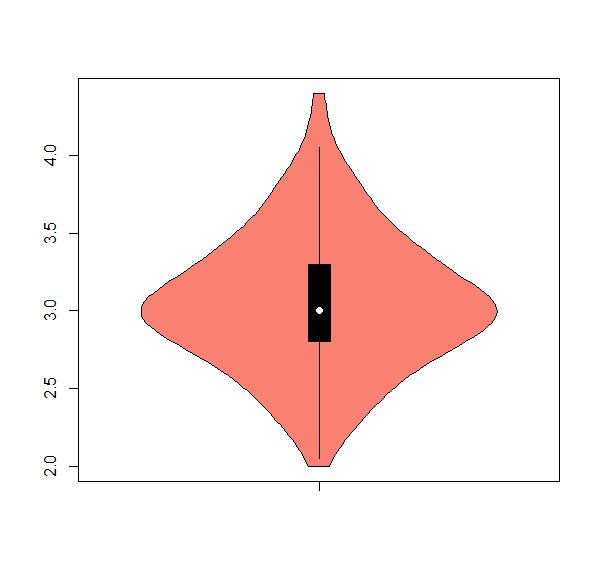
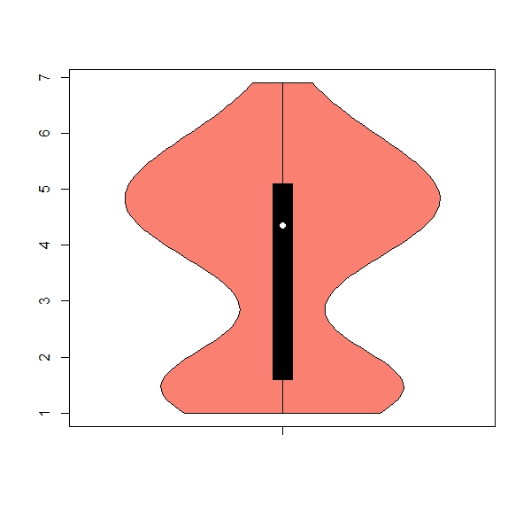
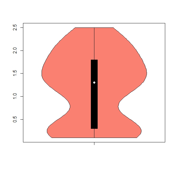
b. The package ‘vioplot’ has a useful function ‘vioplot’ for violin plots (hint: install and activate package). Get one violin plot for each numeric column, remove any numbers from the x axis, color = salmon
Expected results:
apply(iris[,1:4], 2, boxplot)b.
library(vioplot)

apply(iris[,1:4], 2, vioplot, col = "salmon", names = "")
7. Using the ‘apply’ family to work with classes of data.frames
a. Find out which column of iris is not numeric.
b. Identify the levels of the non-numeric column (hint: ‘levels’ function).
c. Try the function “unique” instead, compare the output.
which(sapply(iris, class) != "numeric")b.
levels(iris$Species)c.
unique(iris$Species)"levels" gets you character outputs which are easier to work with, "unique" gets you the original factors
8. Use library ‘ggplot2’, dataset = ‘diamonds’ (hint: install and activate package)
a. Load the library ‘ggplot2’, and dataset ‘diamonds’.
b. Which columns are not numeric in class?.
c. For observations 10000 to 11000, get the mean of columns 8, 9, 10.
d. Same as ‘c’ but round the results to one digit.
e. Sort the rounded results in ascending order.
library(ggplot2)b.
which(sapply(diamonds, class) != "numeric")c.
apply(diamonds[10000:11000, 8:10], 1, mean)d.
round(apply(diamonds[10000:11000, 8:10], 1, mean),1)e.
sort(round(apply(diamonds[10000:11000, 8:10], 1, mean),1)) 9. Function ‘aggregate’
a. Use ‘aggregate’ on ‘mtcars’. Calculate the median for each column sorted by the number of carburetors. Use the standard ‘x’, ‘by’ and ‘FUN’ arguments.
#expected result

  Group.1   mpg cyl   disp  hp  drat    wt   qsec  vs am gear carb
1       1 22.80   4 108.00  93 3.850 2.320 19.470 1.0  1  4.0    1
2       2 22.10   4 143.75 111 3.730 3.170 17.175 0.5  0  4.0    2
3       3 16.40   8 275.80 180 3.070 3.780 17.600 0.0  0  3.0    3
4       4 15.25   8 350.50 210 3.815 3.505 17.220 0.0  0  3.5    4
5       6 19.70   6 145.00 175 3.620 2.770 15.500 0.0  1  5.0    6
6       8 15.00   8 301.00 335 3.540 3.570 14.600 0.0  1  5.0    8
b. Calculate again the median based on ‘carb’, but this time use the ‘formula-dot’ notation.
#expected result

  carb   mpg cyl   disp  hp  drat    wt   qsec  vs am gear
1    1 22.80   4 108.00  93 3.850 2.320 19.470 1.0  1  4.0
2    2 22.10   4 143.75 111 3.730 3.170 17.175 0.5  0  4.0
3    3 16.40   8 275.80 180 3.070 3.780 17.600 0.0  0  3.0
4    4 15.25   8 350.50 210 3.815 3.505 17.220 0.0  0  3.5
5    6 19.70   6 145.00 175 3.620 2.770 15.500 0.0  1  5.0
6    8 15.00   8 301.00 335 3.540 3.570 14.600 0.0  1  5.0
aggregate(x = mtcars, by = list(mtcars$carb), FUN = median)b.
aggregate(. ~ carb, data = mtcars, median) 10. Modulo division in a matrix
a. Get the object ‘mymatrix’ as below
mymatrix = matrix(data = c(6,34,923,5,0, 112:116, 5,9,34,76,2, 545:549), nrow = 5)

> mymatrix
    [,1] [,2] [,3] [,4]
[1,]   6  112    5  545
[2,]  34  113    9  546
[3,] 923  114   34  547
[4,]   5  115   76  548
[5,]   0  116    2  549
c. Use ‘apply’ to perform a modulo division by 10 on each value of the matrix. The new matrix contains the rest of the modulo division.
#expected result

    [,1] [,2] [,3] [,4]
[1,]   6    2    5    5
[2,]   4    3    9    6
[3,]   3    4    4    7
[4,]   5    5    6    8
[5,]   0    6    2    9
mymatrix = matrix(data = c(6,34,923,5,0, 112:116, 5,9,34,76,2, 545:549), nrow = 5)

mymatrix
a.
apply(mymatrix, c(1,2), function(x) x%%10)