
R Exercises for Beginners – 1-10
Practicing is a crucial part of learning a new language. Statistical languages like R are no exception of that rule. Many of my students think the same and would love to see more exercises. Therefore, I decided to write an R exercise sheet for beginners and blog it over here. These R exercises are an add-on to the already existing exercise videos available in each and every R-Tutorial product.
On this sheet you will find 10 R exercises corresponding to the material taught in R Basics and R Level 1. The exercise solutions can be found here in an extra blog post.
I will first write down the exercise question and below the question you can see how the console output should look like. The corresponding code is to be found on the solutions page.
Exercises
1a. Get the length of the “lynx” dataset
[1] 114
1b. Create a vector of ordered “lynx” index numbers (hint: order, increasing)
[1]  69  22  70  71  23  68  99  98  12  78 100  21  79  13  72  59  24  32  60 101  41  42  49
[24]   1  14  40  58   2  88  51  33  30  31  73  89  80  67 102  15  20  61  50 109  11 108  25
[47]  43   3  77 110  97  39  48  34  62  57  81  52  90   4  29 111  26 103  74  82  91  56   5
[70] 107 112  53  44  35  54  19  87  63  38  27  55  16 104  66  28  10 113  17  92  36  64   6
[93]  37 106  95  94  45 114  18  83  76 105  96  86  93   7  75  47  65   9   8  85  46  84
1c. Get 2 vectors (index positions and absolute values) with all “lynx” observations smaller than 500 (hint: which, subset)
[1]   1   2  12  13  14  15  20  21  22  23  24  30  31  32  33  40  41  42  49  50  51  58  59
[24]  60  61  67  68  69  70  71  72  73  78  79  80  88  89  98  99 100 101 102 109
and
[1] 269 321  98 184 279 409 409 151  45  68 213 361 377 225 360 299 236 245 255 473 358 299 201
[24] 229 469 389  73  39  49  59 188 377 105 153 387 345 382  81  80 108 229 399 485
length(lynx)

order(lynx)

which(lynx < 500)

subset(lynx, lynx < 500)
2a. Get a Histogram of the “lynx” dataset
2b. Adjust the bin size to 7 bins
2c. Remove the labs and change the bins to 2 alternating colors
2d. Add a subtitle and divide the main title in 2 lines
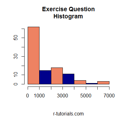
hist(lynx, col=c("salmon2", "darkblue"), breaks=7,

sub="r-tutorials.com", xlab="", ylab="",

main="Exercise Question\nHistogram")
Hint: use \n to get text to next level
3a. Extract Sepal.Length from the “iris” dataset and call the resulting vector mysepal
3b. Get the summation, mean, median, max and min of mysepal
[1] 876.5
[1] 5.843333
[1] 5.8
[1] 4.3
[1] 7.9
3c. Get the summary of mysepal and compare the results with 3b
Min.  1st Qu.  Median    Mean 3rd Qu.    Max.
4.300   5.100   5.800   5.843   6.400   7.900
mysepal = iris$Sepal.Length

sum(mysepal);

mean(mysepal);

median(mysepal);

min(mysepal);

max(mysepal)

summary(mysepal)
4a. Install and load library “dplyr”
4b. Call help for function arrange of “dplyr”
4c. Deinstall “dplyr”
install.packages("dplyr")

library(dplyr)

?arrange

remove.packages("dplyr")
5. Data for this exercise:
x = c(3,6,9)
5a. Repeat x 4 times, but there should be an extra 1 at the end and beginning
[1] 1 3 6 9 3 6 9 3 6 9 3 6 9 1
5b. Call the vector of 5a myvec and extract the 5th value (hint: dplyr, nth)
[1] 3
myvec = c(1, rep(x, times=4), 1)

library(dplyr)

nth(myvec, 5)
6a. Get a subset of “mtcars” with transmission type: manual, and call it mysubset
                mpg cyl  disp  hp drat    wt  qsec vs am gear carb
Mazda RX4      21.0   6 160.0 110 3.90 2.620 16.46  0  1    4    4
Mazda RX4 Wag  21.0   6 160.0 110 3.90 2.875 17.02  0  1    4    4
Datsun 710     22.8   4 108.0  93 3.85 2.320 18.61  1  1    4    1
Fiat 128       32.4   4  78.7  66 4.08 2.200 19.47  1  1    4    1
Honda Civic    30.4   4  75.7  52 4.93 1.615 18.52  1  1    4    2
Toyota Corolla 33.9   4  71.1  65 4.22 1.835 19.90  1  1    4    1
Fiat X1-9      27.3   4  79.0  66 4.08 1.935 18.90  1  1    4    1
Porsche 914-2  26.0   4 120.3  91 4.43 2.140 16.70  0  1    5    2
Lotus Europa   30.4   4  95.1 113 3.77 1.513 16.90  1  1    5    2
Ford Pantera L 15.8   8 351.0 264 4.22 3.170 14.50  0  1    5    4
Ferrari Dino   19.7   6 145.0 175 3.62 2.770 15.50  0  1    5    6
Maserati Bora  15.0   8 301.0 335 3.54 3.570 14.60  0  1    5    8
Volvo 142E     21.4   4 121.0 109 4.11 2.780 18.60  1  1    4    2
6b. Extract the first 2 variables of the first 2 observations of mysubset
              mpg cyl
Mazda RX4      21   6
Mazda RX4 Wag  21   6
mysubset = subset(mtcars, am == 1)

mysubset[c(1,2), c(1,2)]
7a. Get the first 9 observations of “mtcars”
                   mpg cyl  disp  hp drat    wt  qsec vs am gear carb
Mazda RX4         21.0   6 160.0 110 3.90 2.620 16.46  0  1    4    4
Mazda RX4 Wag     21.0   6 160.0 110 3.90 2.875 17.02  0  1    4    4
Datsun 710        22.8   4 108.0  93 3.85 2.320 18.61  1  1    4    1
Hornet 4 Drive    21.4   6 258.0 110 3.08 3.215 19.44  1  0    3    1
Hornet Sportabout 18.7   8 360.0 175 3.15 3.440 17.02  0  0    3    2
Valiant           18.1   6 225.0 105 2.76 3.460 20.22  1  0    3    1
Duster 360        14.3   8 360.0 245 3.21 3.570 15.84  0  0    3    4
Merc 240D         24.4   4 146.7  62 3.69 3.190 20.00  1  0    4    2
Merc 230          22.8   4 140.8  95 3.92 3.150 22.90  1  0    4    2
7b. Get the “mtcars” dataset ordered according to the increasing amount of “carb”
hint for 7b: library dplyr, arrange
head(mtcars, 9)

library(dplyr)

arrange(mtcars, carb)
8a. Get the means of the first 2 columns in the “iris” dataset by Species
iris$Species: setosa
Sepal.Length  Sepal.Width
       5.006        3.428

--------------------------
iris$Species: versicolor
Sepal.Length  Sepal.Width
       5.936        2.770
--------------------------
iris$Species: virginica
Sepal.Length  Sepal.Width
       6.588        2.974
8b. Create vector x which is the alternation of 1 and 2, 75 times, check the length
[1] 1 2 1 2 1 2 1 2 1 2 1 2 1 2 1 2 1 2 1 2 1 2 1 2 1 2 1 2 1 2 1 2 1 2 1 2 1 2 1 2 1 2 1 2 1 2
[47] 1 2 1 2 1 2 1 2 1 2 1 2 1 2 1 2 1 2 1 2 1 2 1 2 1 2 1 2 1 2 1 2 1 2 1 2 1 2 1 2 1 2 1 2 1 2
[93] 1 2 1 2 1 2 1 2 1 2 1 2 1 2 1 2 1 2 1 2 1 2 1 2 1 2 1 2 1 2 1 2 1 2 1 2 1 2 1 2 1 2 1 2 1 2
[139] 1 2 1 2 1 2 1 2 1 2 1 2
8c. Attach x to iris as dataframe “irisx”, check the head
  Sepal.Length Sepal.Width Petal.Length Petal.Width Species x
1          5.1         3.5          1.4         0.2  setosa 1
2          4.9         3.0          1.4         0.2  setosa 2
3          4.7         3.2          1.3         0.2  setosa 1
4          4.6         3.1          1.5         0.2  setosa 2
5          5.0         3.6          1.4         0.2  setosa 1
6          5.4         3.9          1.7         0.4  setosa 2
8d. Get the colsums of columns 1,3,4 in the “irisx” dataset by the new x variable
irisx$x: 1
Sepal.Length Petal.Length  Petal.Width
       438.0        283.2         91.4
---------------------------------------
irisx$x: 2
Sepal.Length Petal.Length  Petal.Width
       438.5        280.5         88.5
by(iris[,1:2], iris$Species, colMeans)

x = rep(1:2, times=75); length(x)

irisx = data.frame(iris, x); head(irisx)

by(irisx[,c(1,3,4)], irisx$x, colSums)
9a. How many observations in “lynx” are smaller than 500?
[1] 43
9b. How many observations in “iris” have a Sepal.Length greater or equal 5?
[1] 128
sum(lynx < 500)

sum(iris$Sepal.Length >= 5)
10a. Plot a simple xy plot with “iris” Sepal.Length vs. Sepal.Width
10b. Enlarge the scale limits: y from 0 – 5, x from 3 – 9
10c. Add a text of your choosing, in red, at the lower part of the plot
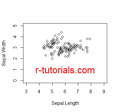
attach(iris)

plot(Sepal.Length, Sepal.Width)

plot(Sepal.Length, Sepal.Width, ylim=c(0,5), xlim=c(3,9))

text(6,1, "r-tutorials.com", col="red", cex=2, lwd=2)