
Pivot Tables – Guest Post from DataJoy
This is a guest post from DataJoy. DataJoy is a zero-installation online R editor ideal for getting started with Data Analysis.
Pivot tables are a powerful tool for summarizing long tables of data where the rows share common attributes. For example, if you had a table of student exam scores with name, sex, year group and score of the student, you could quickly find out things like the average scores for male and female students, or the number of students in each year group. It is also possible to change the structure of the table. For example, you could quickly create a table with a row for each year group, showing average scores in two columns for male and female students. This makes pivot tables a basic but very useful tool for data analysis.
Pivot tables are commonly found in spreadsheets programs, like Microsoft Excel. It is possible to mimic the behavior of pivot tables in R using data frames. We will use the dplyr and tidyr libraries for this.
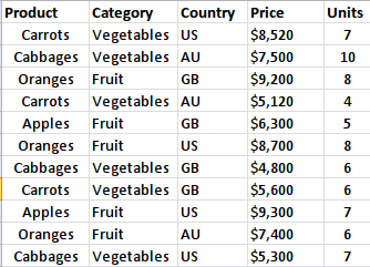
Our example data will be read from a Excel file containing this table:
Summary Tables
Summary tables let us ask questions like “what is average…?”, “what is the total…?”, across different groups.
- First, we read the data from the xlsx file:
library(xlsx)
library(tidyr)
library(dplyr)
products <- read.xlsx("my_data.xlsx",
sheetIndex = 1,
rowIndex = 1:12)
- Now we can manipulate the data. For instance, to see a summary of the product sales:
products <- group_by(products, Category, Product)
sum_product <- summarise(products,
total_price = sum(Price),
total_units = sum(Units))
Which will produce the next table:
| Product|total_price|total_units|
| ------ | ---------:|:---------:|
| Apples |      15600|         12|
| Oranges|      25300|         22|
|Cabbages|      17600|         23|
| Carrots|      19240|         17|
The group_by function allows to perform operations group-wise, determined by variables defined in the data set. The summarize function produces a data frame with extra columns determined by the additional arguments. Common statistical operations can be used with this command like sum, mean,median and sd; we can count the number of occurrences of certain values too with n(). It is also possible to use customized operations.
Suppose we want to add and additional column with the average price for each unit, this is what we have to do:
pivot_product <- summarise(products,
total_price = sum(Price),
total_units = sum(Units),
avg_price = sum(Price)/sum(Units))
And the output of this function is:
| Product |total_price|total_units|avg_price|
| ------- | --------- | --------- | ------- |
| Apples  |      15600|         12|1300.0000|
| Cabbages|      17600|         23| 765.2174|
| Carrots |      19240|         17|1131.7647|
| Oranges |      25300|         22|1150.0000|
We might want to see the information grouped by Country instead. This is easily accomplished changing the argument in the group_by function:
products <- group_by(products, Country)
pivot_product <- summarise(products,
total_price = sum(Price),
total_units = sum(Units),
avg_price = sum(Price)/sum(Units))
This produces:
| Country|total_price|total_units|avg_price|
| ------ | --------- | --------- | ------- |
| AU     |      20020|         20| 1001.000|
| GB     |      25900|         25| 1036.000|
| US     |      31820|         29| 1097.241|
Of course, to summarize the data by Category it is as simple as using that argument in group_by. It is even possible to use more than one variable to group the data. For instance, it might be desirable to summarize the data by Category and Country:
print(head(products))
products <- group_by(products, Category, Country)
pivot_product <- summarise(products,
total_price = sum(Price),
total_units = sum(Units),
avg_price = sum(Price)/sum(Units))
The output is:
| Category  |Country|total_price|total_units|avg_price|
| --------- | ----- | --------- | --------- | ------- |
| Fruit     | AU    |       7400|          6|1233.3333|
| Fruit     | GB    |      15500|         13|1192.3077|
| Fruit     | US    |      18000|         15|1200.0000|
| Vegetables| AU    |      12620|         14| 901.4286|
| Vegetables| GB    |      10400|         12| 866.6667|
| Vegetables| US    |      13820|         14| 987.1429|
Contingency tables
It is also possible to produce cross tabulations as well, for instance, to compare the Product sales for each Country.
- First, we have to summarize the data grouping by Product and Country, and compute the corresponding total price.
pivot_product <- summarise(products,
total_price = sum(Price))
to create this intermediary table:
| Product |Country|total_price|
| ------- | ----- | --------- |
| Apples  | GB    |       6300|
| Apples  | US    |       9300|
| Cabbages| AU    |       7500|
| Cabbages| GB    |       4800|
| Cabbages| US    |       5300|
| Carrots | AU    |       5120|
| Carrots | GB    |       5600|
| Carrots | US    |       8520|
| Oranges | AU    |       7400|
| Oranges | GB    |       9200|
| Oranges | US    |       8700|
No we use the spread() function from the tidyr library to complete the job. It can even handle missing values:
cross_tbl <- spread(pivot_product, Country, total_price)
The final table is
| Product | AU | GB | US |
| ------- | -- | -- | -- |
| Apples  | NA |6300|9300|
| Cabbages|7500|4800|5300|
| Carrots |5120|5600|8520|
| Oranges |7400|9200|8700|
Now we can have a quick view to condensed information and draw conclusions.
Just for the sake of adding a complete example, here is how we can use a contingency table to compare the number of units in each category sold to each country.
library(xlsx)
library(tidyr)
library(dplyr)
products <- read.xlsx("my_data.xlsx",<
sheetIndex = 1,
rowIndex = 1:12)
print(head(products))
products <- group_by(products, Category, Country)
pivot_units <- summarise(products,
total_units = sum(Units))
cross_tbl <- spread(pivot_units, Country, total_units)
print(cross_tbl)
And the corresponding output is:
| Category  |AU|GB|US|
| --------- |--|--|--|
| Fruit     | 6|13|15|
| Vegetables|14|12|14|
There are other libraries that can also produce contingency tables, dcast from reshape2 can be used instead of spread(). Once the data analysis is complete, one can write the resulting tables back to the excel file:
cross_tbl <- data.frame(cross_tbl)
write.xlsx(cross_tbl, "my_data.xlsx",
sheetName="Summarized",
col.names=TRUE,
row.names=FALSE,
append=TRUE,
showNA=TRUE)